数据案例分析

DA Project

2021-04-14

Source

Edit

History

会员用户消费行为浅度挖掘

Catalogue

1. 项目描述
2. 数据导入
3. 数据处理
1. 3.1. 类型转换 & 新字段提取
4. 用户消费分析
5. 用户分层
6. 总结

摘要
通过会员消费数据，分析消费趋势、复购率以及回购率等;并给会员用户进行分层，给后续工作提供数据依据～

项目描述

项目名称：健身平台会员用户消费行为分析

数据来源：数据集来源于网络，是某健身房2019年3月至2020年2月会员消费数据，数据源格式为.xls

字段说明

user_id ：用户ID

order_dt ：购买日期

order_products ：购买数量

order_amount ：购买金额

项目目的：

月度趋势分析
个体消费分析
复购率 & 回购率
用户分层
用户生命周期

数据导入

import pandas as pd
import numpy as np
import matplotlib.pyplot as plt
from datetime import datetime
import os
import warnings

warnings.filterwarnings('ignore')
os.chdir('/home/min/data')
%matplotlib inline

# 可视化风格设定

large = 22
med = 16
small = 13
params = {'axes.titlesize' : large,
         'legend.fontsize' : med,
         'figure.figsize' : (19,10),
         'axes.labelsize' : med,
         'axes.titlesize' : med,
         'xtick.labelsize' : med,
         'ytick.labelsize' : med,
         'figure.titlesize' : large}
plt.rcParams.update(params)
plt.style.use('seaborn-pastel')

1 2	data = pd.read_excel('cuscapi.xls') data.head(10)

	user_id	order_dt	order_products	order_amount
0	vs30033073	2020-01-17	1	20
1	vs30026748	2019-12-04	1	20
2	vs10000716	2019-07-05	1	20
3	vs30032785	2019-08-21	2	0
4	vs10000716	2019-10-24	1	20
5	vs30033073	2019-11-29	2	20
6	vs10000621	2019-07-19	2	20
7	vs30029475	2019-05-17	1	20
8	vs30030664	2019-11-11	1	20
9	vs10000773	2019-11-25	1	20

1	data.info()

<class 'pandas.core.frame.DataFrame'>
RangeIndex: 2013 entries, 0 to 2012
Data columns (total 4 columns):
user_id           2013 non-null object
order_dt          2013 non-null datetime64[ns]
order_products    2013 non-null int64
order_amount      2013 non-null int64
dtypes: datetime64[ns](1), int64(2), object(1)
memory usage: 63.0+ KB

1
2
3

pd.set_option('display.float_format', lambda x : '%.2f' % x)

data.describe()

	order_products	order_amount
count	2013.00	2013.00
mean	1.47	22.90
std	0.91	94.94
min	1.00	0.00
25%	1.00	20.00
50%	1.00	20.00
75%	2.00	20.00
max	12.00	2650.00

图表解析：

用户平均每笔订单购买1.5个商品，标准差为0.9，波动性不大
中位数在1个商品，75分位数在2个产品，说明绝大多数订单的购买数量都不多
平均每笔消费金额为22.9元，标准差约为95，中位数为20，平均数大于中位数，说明多数会员消费金额集中在小金额范围，而小部分会员贡献了大额消费，符号二八法则。

# 根据用户id进行分组汇总


user_group = data.groupby('user_id').sum()
user_group.head(10)

	order_products	order_amount
user_id
vs10000005	9	189
vs10000621	214	5704
vs10000627	2	0
vs10000716	250	2616
vs10000743	1	20
vs10000757	75	1104
vs10000773	23	460
vs10000775	8	2730
vs10000788	7	144
vs10000794	1	0

1	user_group.describe()

	order_products	order_amount
count	247.00	247.00
mean	11.97	186.59
std	36.70	641.12
min	1.00	0.00
25%	2.00	0.00
50%	2.00	0.00
75%	3.00	66.00
max	277.00	5704.00

图表解析：

用户平均购买数量约为12个商品，最多购买了277个商品
平均消费金额约为187元，标准差为641，中位数为0，也说明了存在小部分会员购买了大数量商品的高消费情况

数据处理

类型转换 & 新字段提取

# 类型转换 & 新字段提取(月份)


data['order_dt'] = pd.to_datetime(data['order_dt'])
data['month'] = data['order_dt'].astype('datetime64[M]')
data.head(10)

	user_id	order_dt	order_products	order_amount	month
0	vs30033073	2020-01-17	1	20	2020-01-01
1	vs30026748	2019-12-04	1	20	2019-12-01
2	vs10000716	2019-07-05	1	20	2019-07-01
3	vs30032785	2019-08-21	2	0	2019-08-01
4	vs10000716	2019-10-24	1	20	2019-10-01
5	vs30033073	2019-11-29	2	20	2019-11-01
6	vs10000621	2019-07-19	2	20	2019-07-01
7	vs30029475	2019-05-17	1	20	2019-05-01
8	vs30030664	2019-11-11	1	20	2019-11-01
9	vs10000773	2019-11-25	1	20	2019-11-01

1
2
3

# 检查空值

data.apply(lambda x:sum(x.isnull()))

user_id           0
order_dt          0
order_products    0
order_amount      0
month             0
dtype: int64

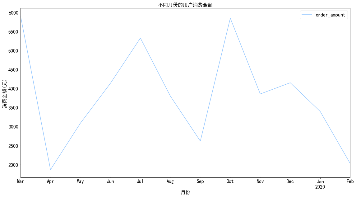
用户消费分析

月度总趋势分析

# 月度消费

data.groupby('month').order_amount.sum().plot()
plt.xlabel('月份')
plt.ylabel('消费金额(元)')
plt.title('不同月份的用户消费金额')
plt.legend()

图表解析：按月份统计每个月的商品消费金额，可以看出，各个月份销量波动起伏较大。

# 月度产品购买数量

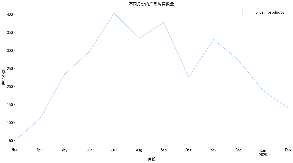
data.groupby('month').order_products.sum().plot()
plt.xlabel('月份')
plt.ylabel('产品个数')
plt.title('不同月份的产品购买数量')
plt.legend()

图表解析：每月的产品购买量呈现为前7个月快速上升，而后5个月呈整体下降的趋势。

# 月度消费次数


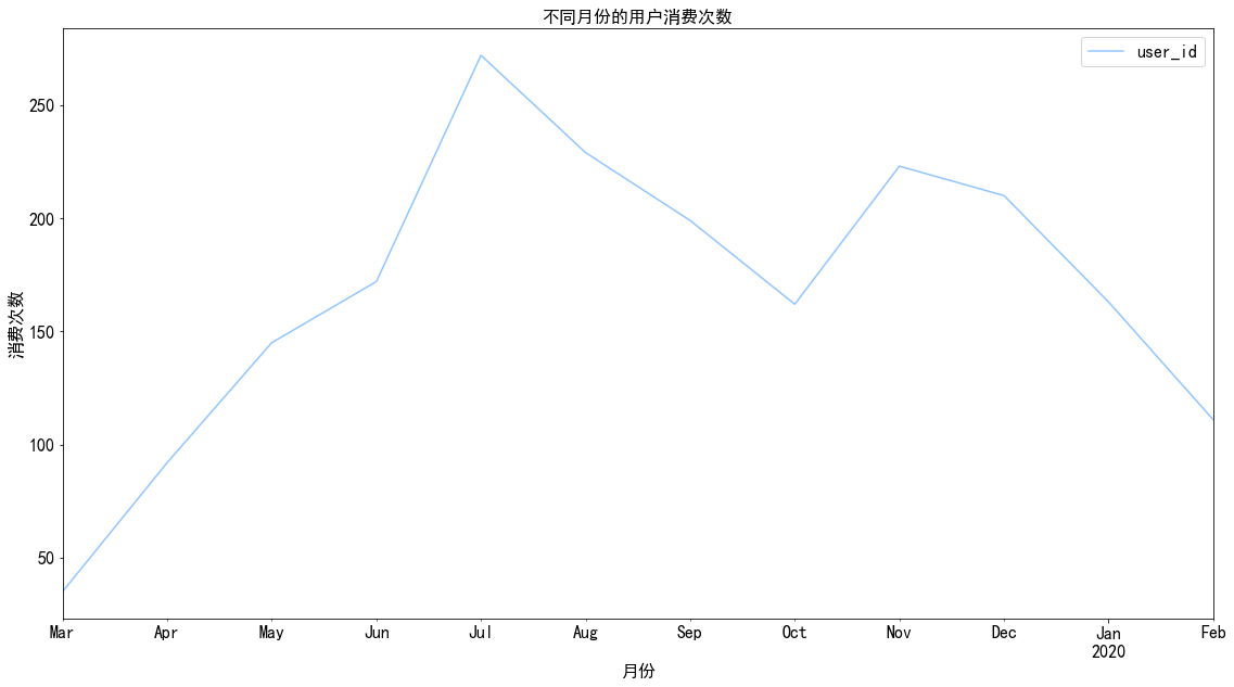
data.groupby('month').user_id.count().plot()
plt.xlabel('月份')
plt.ylabel('消费次数')
plt.title('不同月份的用户消费次数')
plt.legend()

图表解析：消费次数在前四个月呈上升趋势，在六月份达到顶峰，而后呈下降趋势。

# 月度消费人数


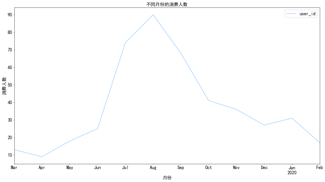
data.groupby('month').user_id.nunique().plot()
plt.xlabel('月份')
plt.ylabel('消费人数')
plt.title('不同月份的消费人数')
plt.legend()

图表解析：相比而言，每月的消费人数大多小于每月的消费人数，而在7月份消费人数达到顶峰90人，后续月份的消费人数持续下降。

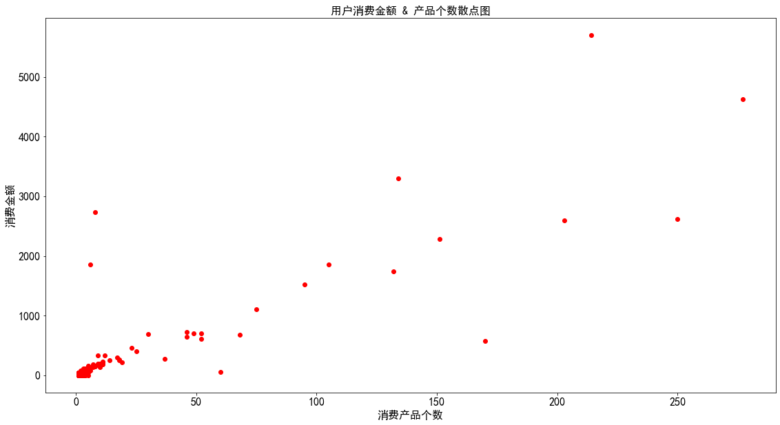
用户个体消费趋势分析

# 用户消费金额 & 产品个数

user_consume = data.groupby('user_id').sum()
plt.scatter(user_consume['order_products'],user_consume['order_amount'],c = 'r')
plt.xlabel('消费产品个数')
plt.ylabel('消费金额')
plt.title('用户消费金额 & 产品个数散点图')

图表解析：可以看到，图中的离散点较多，订单消费金额和订单商品数量的关系不呈线性，用户消费规律性不强，而且订单的极值较多。

# 购买数量分布 & 购买金额分布

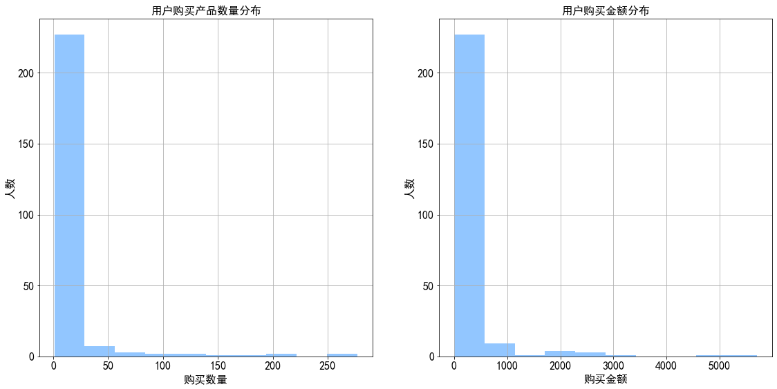
consume_products = user_consume['order_products']
consume_amount = user_consume['order_amount']

fig = plt.figure(figsize = (19,9))
fig.add_subplot(1,2,1)
consume_products.hist(bins = 10)
plt.title('用户购买产品数量分布')
plt.xlabel('购买数量')
plt.ylabel('人数')

fig.add_subplot(1,2,2)
consume_amount.hist(bins = 10)
plt.title('用户购买金额分布')
plt.xlabel('购买金额')
plt.ylabel('人数')

plt.show()

图表解析：大部分用户消费能力不高，图中可知，购买数量大多在50以内，而消费金额大多为1000以内。

# 首次消费会员分布

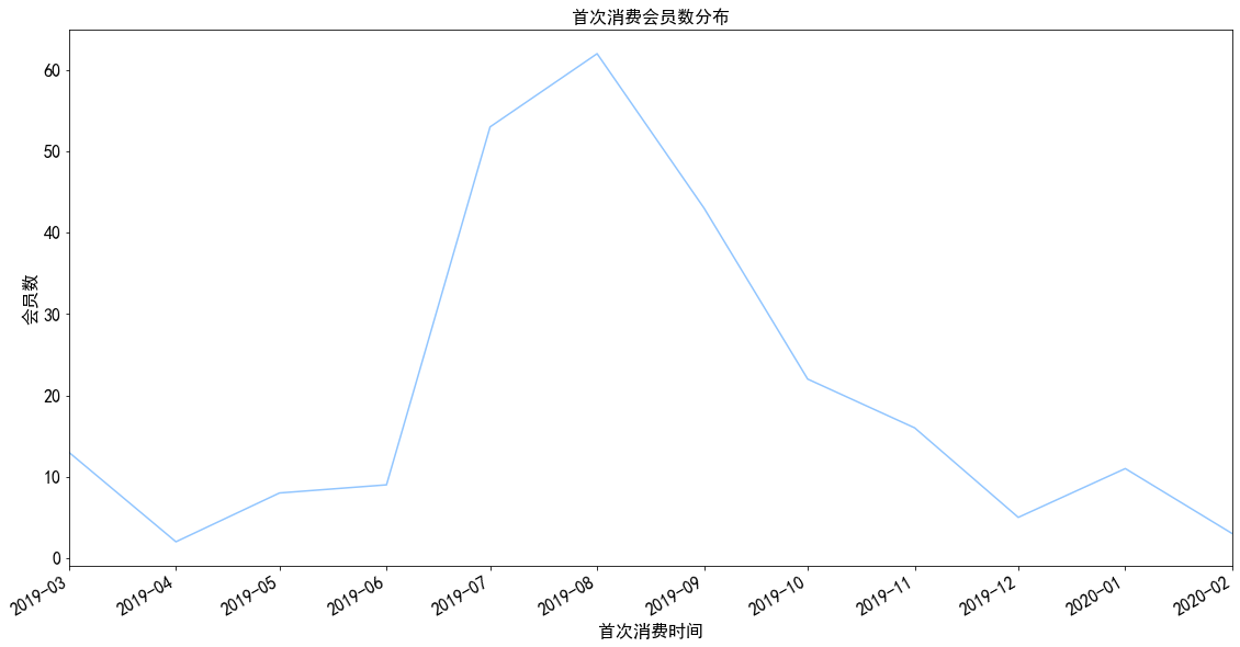
data.groupby('user_id').month.min().value_counts().plot()
plt.title('首次消费会员数分布')
plt.xlabel('首次消费时间')
plt.ylabel('会员数')
plt.show()

# 最后一次消费会员数分析

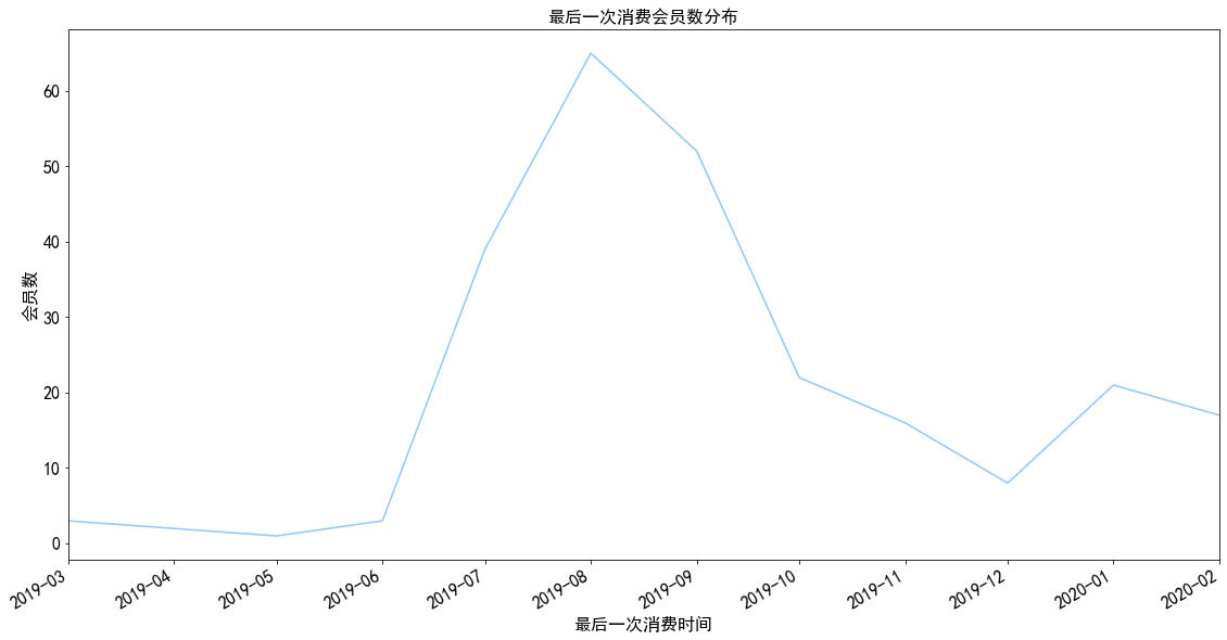
data.groupby('user_id').month.max().value_counts().plot()
plt.title('最后一次消费会员数分布')
plt.xlabel('最后一次消费时间')
plt.ylabel('会员数')
plt.show()

1
2
3

# 首次消费与最后一次消费时间间隔 -- 会员流失情况

(data.groupby('user_id')['month'].agg({'num1':'min','num2':'max'}).num2 - data.groupby('user_id')['month'].agg({'num1':'min','num2':'max'}).num1).value_counts()

0 days      177
31 days      24
61 days       6
92 days       6
122 days      6
337 days      5
30 days       4
306 days      3
153 days      3
184 days      3
62 days       2
123 days      2
215 days      2
245 days      2
275 days      1
276 days      1
dtype: int64

图表解析：

有大量用户的第一次消费集中在7、8月份，有可能是活动引入了大量新用户所导致
相比较最后一次消费，可以观察到大部分用户都在首次消费一个月内流失掉

复购率

# 每位会员各月消费次数

pivoted_counts = data.pivot_table(index='user_id',columns='month',values='order_dt',
                                 aggfunc='count').fillna(0)
columns_month = data.month.sort_values().unique()
pivoted_counts.columns = columns_month
pivoted_counts.head()

	2019-03-01	2019-04-01	2019-05-01	2019-06-01	2019-07-01	2019-08-01	2019-09-01	2019-10-01	2019-11-01	2019-12-01	2020-01-01	2020-02-01
user_id
vs10000005	2.00	0.00	3.00	0.00	0.00	0.00	0.00	0.00	0.00	1.00	0.00	0.00
vs10000621	6.00	17.00	19.00	20.00	17.00	5.00	2.00	18.00	18.00	21.00	16.00	10.00
vs10000627	0.00	0.00	0.00	0.00	2.00	0.00	0.00	0.00	0.00	0.00	0.00	0.00
vs10000716	0.00	0.00	0.00	0.00	14.00	19.00	24.00	12.00	30.00	15.00	12.00	5.00
vs10000743	1.00	0.00	0.00	0.00	0.00	0.00	0.00	0.00	0.00	0.00	0.00	0.00

# 复购定义 ：在某时间段内消费两次或两次以上的会员在总消费会员中的占比
# 时间段 ：月 。 如果一个会员在同一天下了两笔订单，也算作复购用户
# 消费两次及以上记为1，仅消费一次记为0，没有消费记为NaN

pivoted_counts.transf=pivoted_counts.applymap(lambda x:1 if x>1 else np.NaN if x==0 else 0)
pivoted_counts.transf.head()

	2019-03-01	2019-04-01	2019-05-01	2019-06-01	2019-07-01	2019-08-01	2019-09-01	2019-10-01	2019-11-01	2019-12-01	2020-01-01	2020-02-01
user_id
vs10000005	1.00	nan	1.00	nan	nan	nan	nan	nan	nan	0.00	nan	nan
vs10000621	1.00	1.00	1.00	1.00	1.00	1.00	1.00	1.00	1.00	1.00	1.00	1.00
vs10000627	nan	nan	nan	nan	1.00	nan	nan	nan	nan	nan	nan	nan
vs10000716	nan	nan	nan	nan	1.00	1.00	1.00	1.00	1.00	1.00	1.00	1.00
vs10000743	0.00	nan	nan	nan	nan	nan	nan	nan	nan	nan	nan	nan

# 用户复购率分布

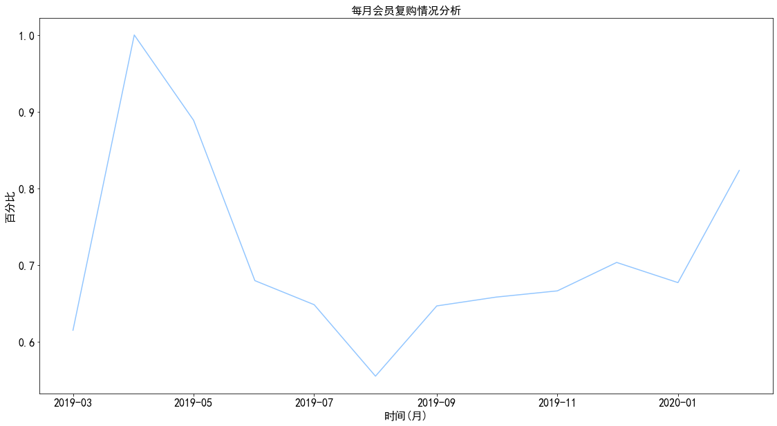
month_counts_rerate = pivoted_counts.transf.sum() / pivoted_counts.transf.count()
plt.plot(month_counts_rerate)
plt.title('每月会员复购情况分析')
plt.xlabel('时间(月)')
plt.ylabel('百分比')
plt.show()

图表解析：

3月份至6月份新用户加入数量较少，复购率上升
在大量新用户加入且大量用户流失的8月份复购率达到最低点
在进行了一波用户流失后，剩余基本为忠实客户，从而使得复购率呈持续上升趋势

# 消费人数和二次消费及以上的用户对比

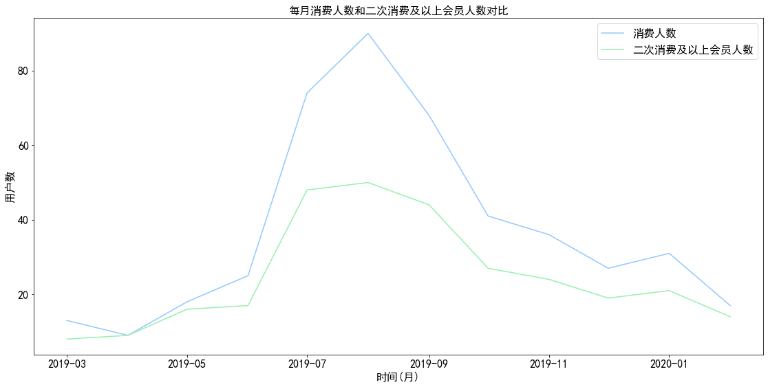
a,b = plt.subplots(figsize=(19,9))
b.plot(pivoted_counts.transf.count())
b.plot(pivoted_counts.transf.sum())
legends = ['消费人数','二次消费及以上会员人数']
plt.title('每月消费人数和二次消费及以上会员人数对比')
plt.xlabel('时间(月)')
plt.ylabel('用户数')
plt.legend(legends)
plt.show()

图表解析：可以看出用户数相差最多的时间节点为八月份，与八月份用户流失有极大关系。但整体趋势保持一致。

回购率

# 回购率 -- 某一时间段内消费的用户，在下一时间段仍然消费的占比
# 实例：如1月消费用户1000,1000中有300个2月依然消费，回购率为30%

pivoted_amount = data.pivot_table(index='user_id',columns='month',
                                 values='order_amount',aggfunc='mean').fillna(0)
pivoted_amount.columns = columns_month
pivoted_amount.head()

	2019-03-01	2019-04-01	2019-05-01	2019-06-01	2019-07-01	2019-08-01	2019-09-01	2019-10-01	2019-11-01	2019-12-01	2020-01-01	2020-02-01
user_id
vs10000005	25.00	0.00	19.67	0.00	0.00	0.00	0.00	0.00	0.00	80.00	0.00	0.00
vs10000621	414.00	20.00	20.00	20.00	17.65	20.00	20.00	20.00	20.00	20.00	20.00	20.00
vs10000627	0.00	0.00	0.00	0.00	0.00	0.00	0.00	0.00	0.00	0.00	0.00	0.00
vs10000716	0.00	0.00	0.00	0.00	20.00	41.84	10.83	15.00	15.33	20.00	20.00	20.20
vs10000743	20.00	0.00	0.00	0.00	0.00	0.00	0.00	0.00	0.00	0.00	0.00	0.00

# 统计有回购的会员人数

pivoted_purchase = pivoted_amount.applymap(lambda x:1 if x>1 else 0)
pivoted_purchase.head()

	2019-03-01	2019-04-01	2019-05-01	2019-06-01	2019-07-01	2019-08-01	2019-09-01	2019-10-01	2019-11-01	2019-12-01	2020-01-01	2020-02-01
user_id
vs10000005	1	0	1	0	0	0	0	0	0	1	0	0
vs10000621	1	1	1	1	1	1	1	1	1	1	1	1
vs10000627	0	0	0	0	0	0	0	0	0	0	0	0
vs10000716	0	0	0	0	1	1	1	1	1	1	1	1
vs10000743	1	0	0	0	0	0	0	0	0	0	0	0

def purchase_reture(data):
    status = []
    for i in range(11):
        if data[i] >= 1:
            if data[i+1] >= 1:
                status.append(1)
            else:
                status.append(0)
        else:
            status.append(np.NaN)
    status.append(np.NaN)
    return pd.Series(status)

1
2
3

pivoted_purchase_reture = pivoted_purchase.apply(purchase_reture,axis = 1)
pivoted_purchase_reture.columns = columns_month
pivoted_purchase_reture.head()

	2019-03-01	2019-04-01	2019-05-01	2019-06-01	2019-07-01	2019-08-01	2019-09-01	2019-10-01	2019-11-01	2019-12-01	2020-01-01	2020-02-01
user_id
vs10000005	0.00	nan	0.00	nan	nan	nan	nan	nan	nan	0.00	nan	nan
vs10000621	1.00	1.00	1.00	1.00	1.00	1.00	1.00	1.00	1.00	1.00	1.00	nan
vs10000627	nan	nan	nan	nan	nan	nan	nan	nan	nan	nan	nan	nan
vs10000716	nan	nan	nan	nan	1.00	1.00	1.00	1.00	1.00	1.00	1.00	nan
vs10000743	0.00	nan	nan	nan	nan	nan	nan	nan	nan	nan	nan	nan

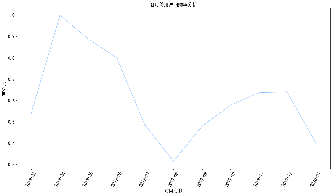
pivoted_purchase_reture_rate = pivoted_purchase_reture.sum() / pivoted_purchase_reture.count()
plt.plot(pivoted_purchase_reture_rate)
plt.title('各月份用户回购率分析')
plt.xlabel('时间(月)')
plt.ylabel('百分比')
plt.xticks(rotation = 60)
plt.show()

图表解析：

用户回购率在4月份达到顶峰，而后呈下降趋势，至8月份到达最低点，原因有可能是用户在4月份至八月份的持续流失所导致
八月份往后，回购率由于剩余的忠实用户所呈上升趋势

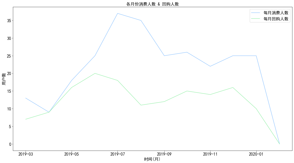
a,b = plt.subplots(figsize = (19,10))
b.plot(pivoted_purchase_reture.count())
b.plot(pivoted_purchase_reture.sum())
legends = ['每月消费人数','每月回购人数']
b.legend(legends)
plt.title('各月份消费人数 & 回购人数')
plt.xlabel('时间(月)')
plt.ylabel('用户数')
plt.show()

图表解析：回购人数变化趋势基本与每月消费人数变化趋势保持一致。

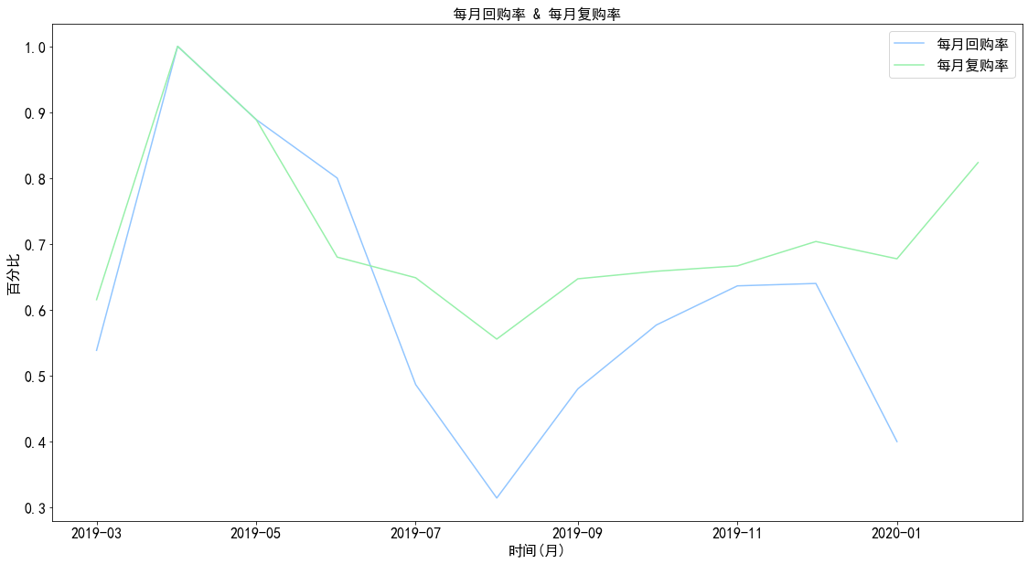
a,b = plt.subplots(figsize = (19,10))
b.plot(pivoted_purchase_reture_rate)
b.plot(month_counts_rerate)
legends = ['每月回购率','每月复购率']
b.legend(legends)
plt.title('每月回购率 & 每月复购率')
plt.xlabel('时间(月)')
plt.ylabel('百分比')
plt.show()

图表解析：

大体上来看，每月用户的复购率高于回购率，波动性也比较大

用户分层

RFM 分层

user_rfm = data.pivot_table(index='user_id',
                           values=['order_dt','order_products','order_amount'],
                           aggfunc={'order_dt':'max','order_products':'count',
                                   'order_amount':'sum'})
user_rfm['order_dt'] = pd.to_datetime(user_rfm['order_dt']).dt.normalize()
user_rfm.head()

	order_amount	order_dt	order_products
user_id
vs10000005	189	2019-12-27	6
vs10000621	5704	2020-02-28	169
vs10000627	0	2019-07-23	2
vs10000716	2616	2020-02-28	131
vs10000743	20	2019-03-15	1

1
2
3

user_rfm['period'] = (user_rfm.order_dt.max() - user_rfm.order_dt) / np.timedelta64(1,'D')
user_rfm = user_rfm.rename(columns={'period':'R','order_products':'F','order_amount':'M'})
user_rfm.head()

	M	order_dt	F	R
user_id
vs10000005	189	2019-12-27	6	63.00
vs10000621	5704	2020-02-28	169	0.00
vs10000627	0	2019-07-23	2	220.00
vs10000716	2616	2020-02-28	131	0.00
vs10000743	20	2019-03-15	1	350.00

# 分层函数定义

def rfm_func(x):
    level = x.apply(lambda x:'1' if x>=0 else '0')
    label = level.R + level.F + level.M
    d = {'111':'高价值客户','011':'重点保持客户',
        '101':'重点发展客户','001':'重点挽留客户',
        '110':'一般价值客户','010':'一般保持客户',
        '100':'一般发展客户','000':'潜在客户'}
    result = d[label]
    return result
user_rfm['label'] = user_rfm[['R','F','M']].apply(lambda x:x-x.mean()).apply(rfm_func,
                                                                            axis = 1)
user_rfm.head()

	M	order_dt	F	R	label
user_id
vs10000005	189	2019-12-27	6	63.00	重点挽留客户
vs10000621	5704	2020-02-28	169	0.00	重点保持客户
vs10000627	0	2019-07-23	2	220.00	一般发展客户
vs10000716	2616	2020-02-28	131	0.00	重点保持客户
vs10000743	20	2019-03-15	1	350.00	一般发展客户

1	user_rfm.groupby('label').count()

	M	order_dt	F	R
label
一般保持客户	3	3	3	3
一般发展客户	146	146	146	146
潜在客户	63	63	63	63
重点保持客户	24	24	24	24
重点发展客户	2	2	2	2
重点挽留客户	2	2	2	2
高价值客户	7	7	7	7

1	user_rfm.groupby('label').sum()

	M	F	R
label
一般保持客户	352	34	98.00
一般发展客户	2653	272	28793.00
潜在客户	1723	125	6377.00
重点保持客户	32494	1416	846.00
重点发展客户	2091	5	575.00
重点挽留客户	2919	9	165.00
高价值客户	3856	152	1429.00

# 字体管理
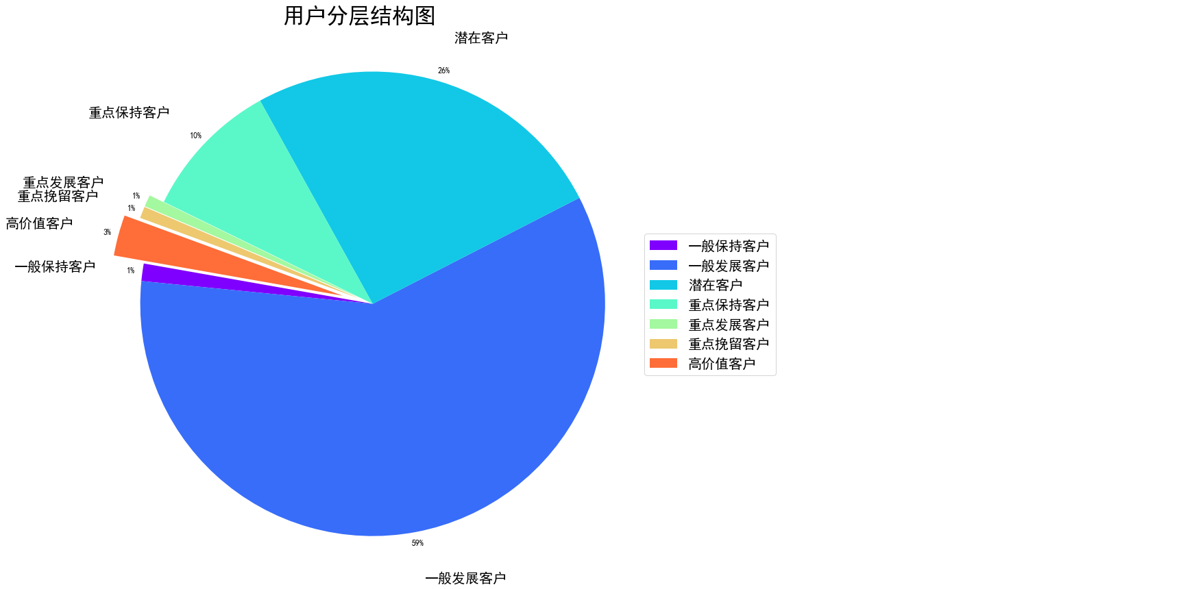
from matplotlib import font_manager as fm

# 颜色
from matplotlib import cm

proptease = fm.FontProperties()
proptease.set_size(20)

labelindex = user_rfm.groupby('label').count().index
labelvalues = user_rfm.groupby('label')['M'].count().tolist()
s = pd.Series(labelvalues,index=labelindex)
labels = s.index
sizes = s.values

explode = (0,0,0,0,0.1,0.1,0.2)
fig,axes = plt.subplots(1,2,figsize = (24,12))
ax1,ax2 = axes.ravel()

colors = cm.rainbow(np.arange(len(sizes)) / len(sizes))
patches,texts,autotests = ax1.pie(sizes,labels = labels,autopct = '%1.0f%%',
                                 explode = explode,shadow = False, startangle = 170,
                                 colors = colors,labeldistance = 1.2,
                                 pctdistance = 1.05,radius = 1.5)
ax1.axis('equal')
plt.setp(texts,fontproperties = proptease)

for i in autotests:
    i.set_size('larger')
ax1.set_title('用户分层结构图',loc = 'center',fontsize = 32)
ax2.axis('off')
ax2.legend(patches,labels,loc = 'center left',fontsize = 20)
plt.tight_layout()
plt.show()

图表解析：

由图可知，一般发展客户占了较大的占比，为59%
潜在客户占比为26%，位居第二，而重点挽留客户以及重点发展客户均只占1%，需要对潜在客户进行引导及转化为忠实用户

根据活跃度分层

# 根据消费行为，简单划分为：新用户、活跃用户、不活跃用户、回流用户

# 新用户 -- 第一次消费
# 活跃用户 -- 老客户，在某一时间区间有过消费
# 不活跃用户 -- 在设定时间区间内没有消费的老客户
# 回流用户 -- 在上一设定时间区间内没有消费，在当前时间区间内有消费

# 时间区间设定为以月为单位统计

def active_stauts(data):
    status = []
    for i in range(12):
        # 本月没有消费
        if data[i] == 0:
            if len(status) > 0:
                if status[i-1] == 'unreg':
                    status.append('unreg')
                else:
                    status.append('unactive')
            else:
                status.append('unreg')
        else:
            if len(status) == 0:
                status.append('new')
            else:
                if status[i-1] == 'unactive':
                    status.append('return')
                elif status[i-1] == 'unreg':
                    status.append('new')
                else:
                    status.append('active')
    return pd.Series(status)

pivoted_purchase_status = pivoted_purchase.apply(lambda x:active_stauts(x),axis = 1)
pivoted_purchase_status.columns = columns_month
pivoted_purchase_status.head()

	2019-03-01	2019-04-01	2019-05-01	2019-06-01	2019-07-01	2019-08-01	2019-09-01	2019-10-01	2019-11-01	2019-12-01	2020-01-01	2020-02-01
user_id
vs10000005	new	unactive	return	unactive	unactive	unactive	unactive	unactive	unactive	return	unactive	unactive
vs10000621	new	active	active	active	active	active	active	active	active	active	active	active
vs10000627	unreg	unreg	unreg	unreg	unreg	unreg	unreg	unreg	unreg	unreg	unreg	unreg
vs10000716	unreg	unreg	unreg	unreg	new	active	active	active	active	active	active	active
vs10000743	new	unactive	unactive	unactive	unactive	unactive	unactive	unactive	unactive	unactive	unactive	unactive

1 2	pivoted_status_counts = pivoted_purchase_status.replace('unreg',np.NaN).apply(lambda x:pd.value_counts(x)) pivoted_status_counts.head()

	2019-03-01	2019-04-01	2019-05-01	2019-06-01	2019-07-01	2019-08-01	2019-09-01	2019-10-01	2019-11-01	2019-12-01	2020-01-01	2020-02-01
active	nan	7.00	9	16.00	20.00	18.00	11	12	15	14	16	10
new	13.00	2.00	8	9.00	17.00	17.00	10	9	6	7	7	1
return	nan	nan	1	nan	nan	nan	4	5	1	4	2	3
unactive	nan	6.00	5	7.00	12.00	31.00	51	59	69	73	80	92

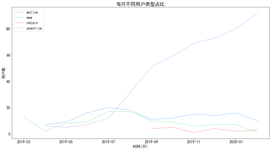
plt.plot(pivoted_status_counts.T)
plt.title('每月不同用户类型占比',fontsize = 20)
plt.legend(pivoted_status_counts.index)
plt.xlabel('时间(月)')
plt.ylabel('用户数')
plt.show()

图表解析：

可以看到，不活跃用户占了较大的比重，而且呈持续上升趋势
活跃用户为蓝色部分，保持较为稳定的状态，而回流用户在9月份产生并维持稳定，但回流人数并不高

# 回流用户 & 活跃用户


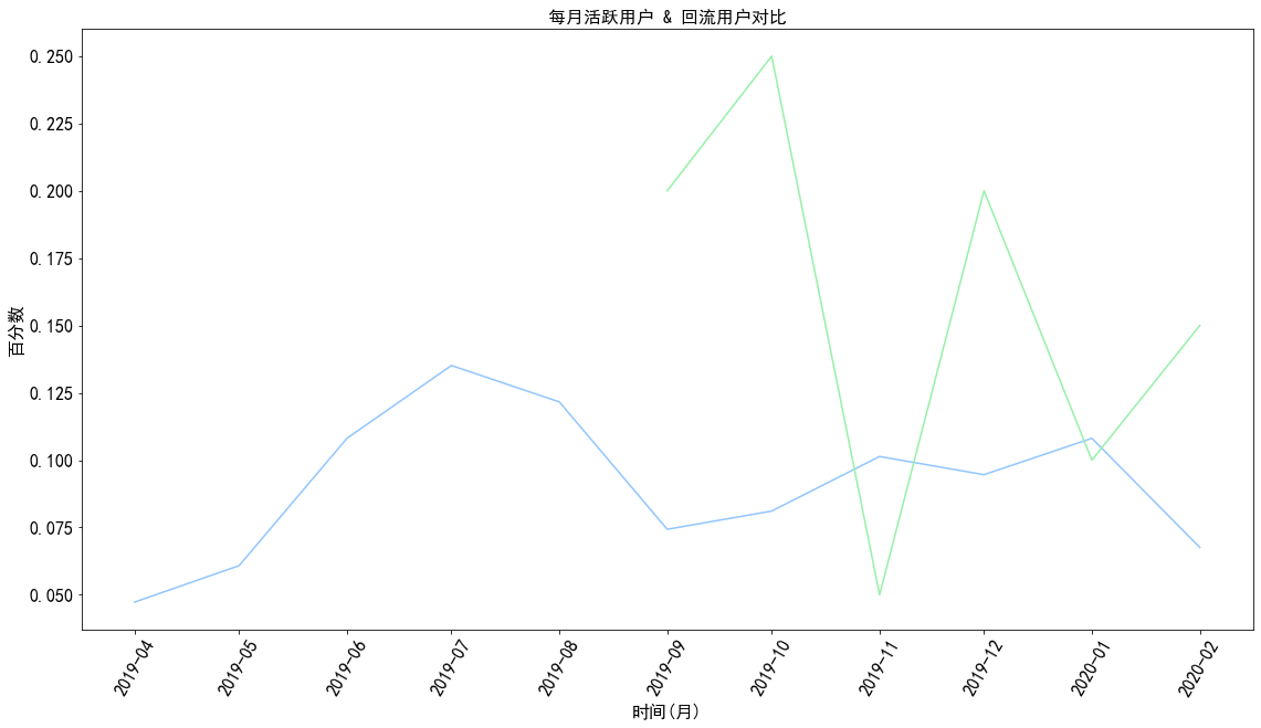
return_rate = pivoted_status_counts.apply(lambda x:x/x.sum(),axis = 1)
plt.plot(return_rate.loc[['active','return'],].T)
plt.title('每月活跃用户 & 回流用户对比')
plt.xlabel('时间(月)')
plt.ylabel('百分数')
plt.xticks(rotation = 60)
plt.show()

图表解析：结合回流用户和活跃用户来看，在后期消费用户中，约70%是回流用户，30%为活跃用户，整体用户质量较好。

用户质量

1
2
3

user_amount = data.groupby('user_id').order_amount.sum().sort_values().reset_index()
user_amount['amount_cumsum'] = user_amount.order_amount.cumsum()
user_amount.tail()

	user_id	order_amount	amount_cumsum
242	vs10000716	2616	29735
243	vs10000775	2730	32465
244	vs30026748	3296	35761
245	vs30029475	4623	40384
246	vs10000621	5704	46088

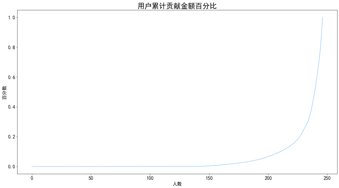
amount_total = user_amount.amount_cumsum.max()
user_amount['prop'] = user_amount.amount_cumsum.apply(lambda x:x/amount_total)
plt.plot(user_amount.prop)
plt.title('用户累计贡献金额百分比',fontsize = 24)
plt.xlabel('人数')
plt.ylabel('百分数')
plt.show()

图表解析：数据集用户共247人，其中约50人贡献了超过80%的销售额，也符合二八定律。

用户生命周期

# 各会员首次 & 最后一次消费时间间隔

order_dt_min = data.groupby('user_id').order_dt.min().dt.date
order_dt_max = data.groupby('user_id').order_dt.max().dt.date
life_time = (order_dt_max - order_dt_min).reset_index()
life_time.head()

	user_id	order_dt
0	vs10000005	273 days
1	vs10000621	351 days
2	vs10000627	1 days
3	vs10000716	238 days
4	vs10000743	0 days

1	life_time.describe()

	order_dt
count	247
mean	32 days 03:59:01.700404
std	73 days 19:15:10.251372
min	0 days 00:00:00
25%	0 days 00:00:00
50%	1 days 00:00:00
75%	13 days 00:00:00
max	351 days 00:00:00

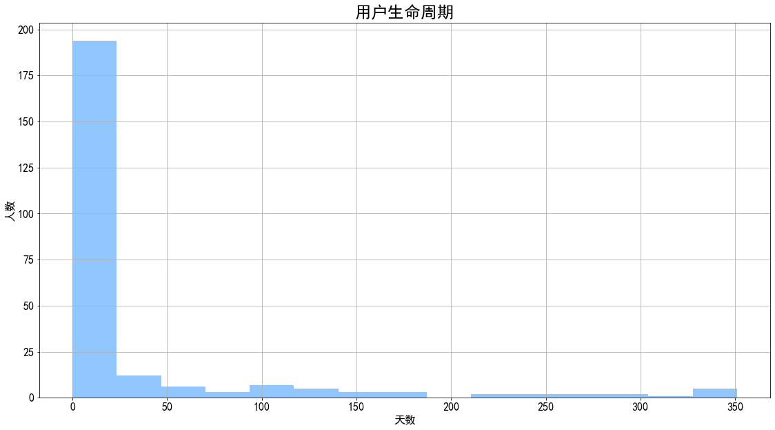
((order_dt_max - order_dt_min) / np.timedelta64(1,'D')).hist(bins = 15)
plt.title('用户生命周期',fontsize = 24)
plt.xlabel('天数')
plt.ylabel('人数')
plt.show()

图表解析：

用户平均生命周期为32天，中位数为1天，说明存在至少50%的客户的首次消费即最后一次消费。
最大生命周期为351天，约为数据源总时间长度，说明存在了从开始到最后有进行了消费的高质量用户

#  消费两次及以上的用户生命周期


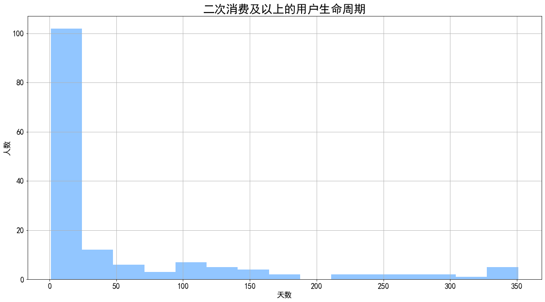
life_time['life_time'] = life_time.order_dt / np.timedelta64(1,'D')
life_time[life_time.life_time > 0].life_time.hist(bins = 15)
plt.title('二次消费及以上的用户生命周期',fontsize = 24)
plt.xlabel('天数')
plt.ylabel('人数')
plt.show()

1	life_time[life_time.life_time > 0].life_time.describe()

count   155.00
mean     51.26
std      87.84
min       1.00
25%       2.00
50%       7.00
75%      53.50
max     351.00
Name: life_time, dtype: float64

图表解析：

二次消费及以上用户生命周期为51天，高于总体用户生命周期。
从营销策略上看，用户在进行了首次消费后，需要对其进行引导再次消费，时间区间应该在30天之内。

用户留存率

# 留存率 --> 用户在第一次消费后，有多少比率进行了第二次消费
# 与回流率的区别在于：留存倾向计算第一次消费，并有多个时间区间

user_purchase_retention = pd.merge(left=data,right = order_dt_min.reset_index(),
                                  how = 'inner',on = 'user_id',suffixes=('','_min'))
user_purchase_retention['order_dt'] = pd.to_datetime(user_purchase_retention['order_dt'])
user_purchase_retention['order_dt_min'] = pd.to_datetime(user_purchase_retention['order_dt_min'])
user_purchase_retention['date_diff'] = (user_purchase_retention.order_dt - user_purchase_retention.order_dt_min) / np.timedelta64(1,'D')
bin = [0,30,60,90,120,150,180,365]
user_purchase_retention['date_diff_bin'] = pd.cut(user_purchase_retention['date_diff'],bins = bin)
user_purchase_retention.head()

	user_id	order_dt	order_products	order_amount	month	order_dt_min	date_diff	date_diff_bin
0	vs30033073	2020-01-17	1	20	2020-01-01	2019-09-23	116.00	(90, 120]
1	vs30033073	2019-11-29	2	20	2019-11-01	2019-09-23	67.00	(60, 90]
2	vs30033073	2019-11-13	2	20	2019-11-01	2019-09-23	51.00	(30, 60]
3	vs30033073	2019-12-24	2	20	2019-12-01	2019-09-23	92.00	(90, 120]
4	vs30033073	2019-10-29	2	20	2019-10-01	2019-09-23	36.00	(30, 60]

pivoted_retention = user_purchase_retention.pivot_table(index='user_id',
                                                       columns = 'date_diff_bin',
                                                       values='order_amount',
                                                       aggfunc=sum,
                                                       dropna=False)
pivoted_retention.head()

date_diff_bin	(0, 30]	(30, 60]	(60, 90]	(90, 120]	(120, 150]	(150, 180]	(180, 365]
user_id
vs10000005	17.00	59.00	nan	nan	nan	nan	80.00
vs10000621	240.00	280.00	440.00	400.00	200.00	40.00	1700.00
vs10000627	0.00	nan	nan	nan	nan	nan	nan
vs10000716	280.00	795.00	240.00	220.00	420.00	300.00	341.00
vs10000743	nan	nan	nan	nan	nan	nan	nan

1	pivoted_retention.mean()

date_diff_bin
(0, 30]       47.88
(30, 60]     148.62
(60, 90]     169.92
(90, 120]    310.32
(120, 150]   112.90
(150, 180]   112.93
(180, 365]   700.36
dtype: float64

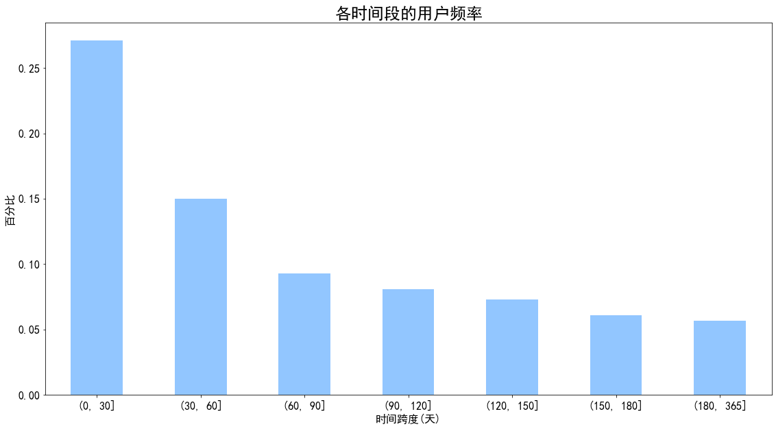
pivoted_retention.transf = pivoted_retention.fillna(0).applymap(lambda x:1 if x>0 else 0)
(pivoted_retention.transf.sum() / pivoted_retention.transf.count()).plot.bar()
plt.title('各时间段的用户频率',fontsize = 24)
plt.xlabel('时间跨度(天)')
plt.xticks(rotation = 360)
plt.ylabel('百分比')
plt.show()

图表解析：

第一个月留存率超过了25%，而第二个月下降至15%左右
之后几个月的留存率基本稳定在5%~10%之间，说明后面第二个月开始的流失率较大，且呈持续流失状态

# 消费召回分析


def diff(group):
    d = group.date_diff.shift(-1) - group.date_diff
    return d

last_diff = user_purchase_retention.sort_values('order_dt').reset_index().groupby('user_id').apply(diff)
last_diff.head()

user_id        
vs10000005  32      0.40
            33     41.60
            155     1.00
            160     0.46
            161   230.16
Name: date_diff, dtype: float64

1	last_diff.describe()

count   1766.00
mean       4.50
std       14.03
min        0.00
25%        0.81
50%        1.43
75%        3.57
max      230.16
Name: date_diff, dtype: float64

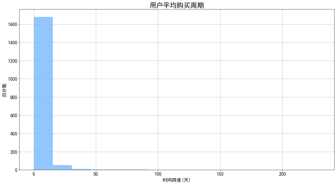
last_diff.hist(bins = 15)
plt.title('用户平均购买周期',fontsize = 23)
plt.xlabel('时间跨度(天)')
plt.ylabel('百分数')
plt.show()

图表解析：

图像呈典型的长尾分布，说明大部分的用户消费时间间隔短
从统计数据来看，用户平均消费间隔为4.5天，说明需要在4.5天左右的消费间隔对用户进行引导召回

总结

以上为健身平台用户消费行为分析的全部内容，感谢阅读。