摘要
上篇文章介绍了数据分布情况的可视化的四种图表 (直方图、密度图、柱状图、折线图)的 展示方法,下面将介绍另外几种直观显示数据分布情况的可视化图表
也称为「点图」、「散布图」或「X-Y 点图」。
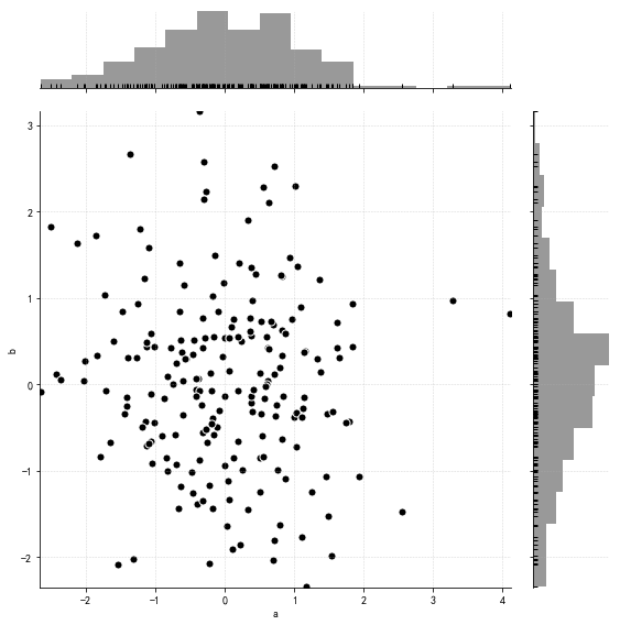
所谓的散点图 (Scatterplot) 就是在笛卡尔座标上放置一系列的数据点,用来显示两个变量的数值(每个轴上显示一个变量),并检测两个变量之间的关系或相关性是否存在。
可以很直观的观察到数据的分布情况
1
2
3
4
5
6
7
8
9
10
import pandas as pdimport numpy as npimport matplotlib.pyplot as pltimport seaborn as sns%matplotlib inline import warningswarnings.filterwarnings('ignore' )
1 2 3 4 5 6 7 8 9 10 11 12 13 14 15 16 17 18 19 rs = np.random.RandomState(2 ) df = pd.DataFrame(rs.randn(200 ,2 ),columns = ['a' ,'b' ]) sns.jointplot(x = df['a' ],y = df['b' ], data = df, color = 'k' , s = 50 ,edgecolor = 'w' ,linewidth = 1 , kind = 'scatter' , space = 0.3 , size = 8 , ratio = 5 , marginal_kws = dict (bins = 15 ,rug = True ) )
<seaborn.axisgrid.JointGrid at 0x5759510>
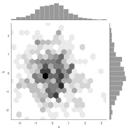
1 2 3 4 5 6 7 8 df = pd.DataFrame(rs.randn(500 ,2 ),columns = ['a' ,'b' ]) with sns.axes_style('white' ): sns.jointplot(x = df['a' ],y = df['b' ],kind = 'hex' , color = 'k' , marginal_kws = dict (bins = 20 ))
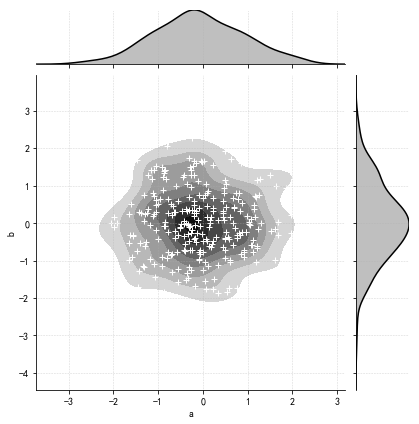
1 2 3 4 5 6 7 8 9 10 rs = np.random.RandomState(15 ) df = pd.DataFrame(rs.randn(300 ,2 ),columns = ['a' ,'b' ]) g = sns.jointplot(x = df['a' ],y = df['b' ],data = df, kind = 'kde' , color = 'k' , shade_lowest = False ) g.plot_joint(plt.scatter,c = 'w' , s = 30 ,linewidth = 1 ,marker = '+' )
<seaborn.axisgrid.JointGrid at 0x1431ec90>
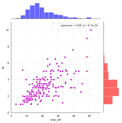
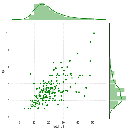
1 2 3 4 5 6 7 8 9 10 11 12 13 14 15 16 17 18 19 20 sns.set_style('white' ) tips = sns.load_dataset('tips' ) print ('tips.head()' )g = sns.JointGrid(x = 'total_bill' ,y = 'tip' ,data = tips) g.plot_joint(plt.scatter,color = 'm' ,edgecolor = 'white' ) g.ax_marg_x.hist(tips['total_bill' ],color = 'b' ,alpha = 0.6 , bins = np.arange(0 ,60 ,3 )) g.ax_marg_y.hist(tips['tip' ],color = 'r' ,alpha = 0.6 , orientation = 'horizontal' ,bins = np.arange(0 ,12 ,1 )) from scipy import statsg.annotate(stats.pearsonr) plt.grid(linestyle = '--' )
分别绘制散点图和直方图
1 2 3 4 5 6 7 8 9 10 11 g = sns.JointGrid(x = 'total_bill' , y = 'tip' , data = tips) g = g.plot_joint(plt.scatter,color = 'g' ,s = 40 ,edgecolor = 'white' ) plt.grid(linestyle = '--' ) g.plot_marginals(sns.distplot,kde = True ,color = 'g' )
<seaborn.axisgrid.JointGrid at 0x154c0690>
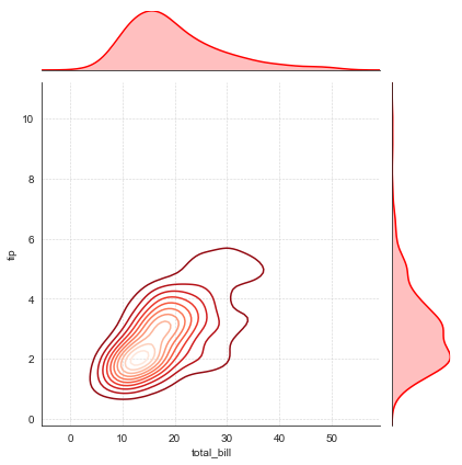
分别绘制密度图和面积图
1 2 3 4 5 6 7 8 9 10 11 g = sns.JointGrid(x = 'total_bill' , y = 'tip' , data = tips) g = g.plot_joint(sns.kdeplot,cmap = 'Reds_r' ) plt.grid(linestyle = '--' ) g.plot_marginals(sns.kdeplot,shade = True ,color = 'r' )
<seaborn.axisgrid.JointGrid at 0x154b13b0>
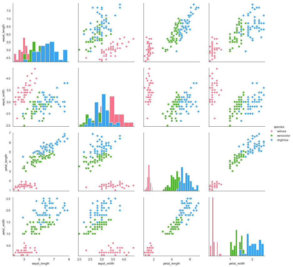
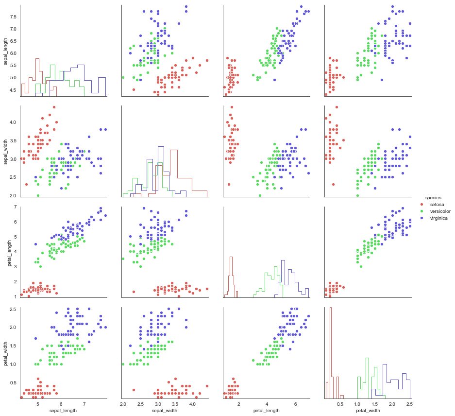
散点图矩阵是组织成网格(矩阵)形式的散点图集合。每个散点图显示一对变量之间的关系。
1 2 3 4 5 6 7 8 9 10 11 12 13 14 15 16 17 18 19 20 21 22 23 24 25 26 27 sns.set_style('white' ) iris = sns.load_dataset('iris' ) print (iris.head())sns.pairplot(iris, kind = 'scatter' , diag_kind = 'hist' , hue = 'species' , palette = 'husl' , markers = ['o' ,'s' ,'D' ], size = 3 )
   sepal_length  sepal_width  petal_length  petal_width species
0           5.1          3.5           1.4          0.2  setosa
1           4.9          3.0           1.4          0.2  setosa
2           4.7          3.2           1.3          0.2  setosa
3           4.6          3.1           1.5          0.2  setosa
4           5.0          3.6           1.4          0.2  setosa

<seaborn.axisgrid.PairGrid at 0x15511310>
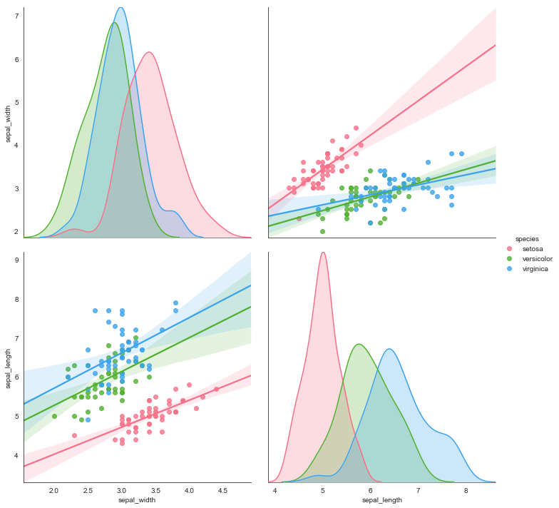
1 2 3 4 5 sns.pairplot(iris,vars = ['sepal_width' ,'sepal_length' ], kind = 'reg' ,diag_kind = 'kde' , hue = 'species' ,palette = 'husl' ,size = 5 )
<seaborn.axisgrid.PairGrid at 0x1d94b510>
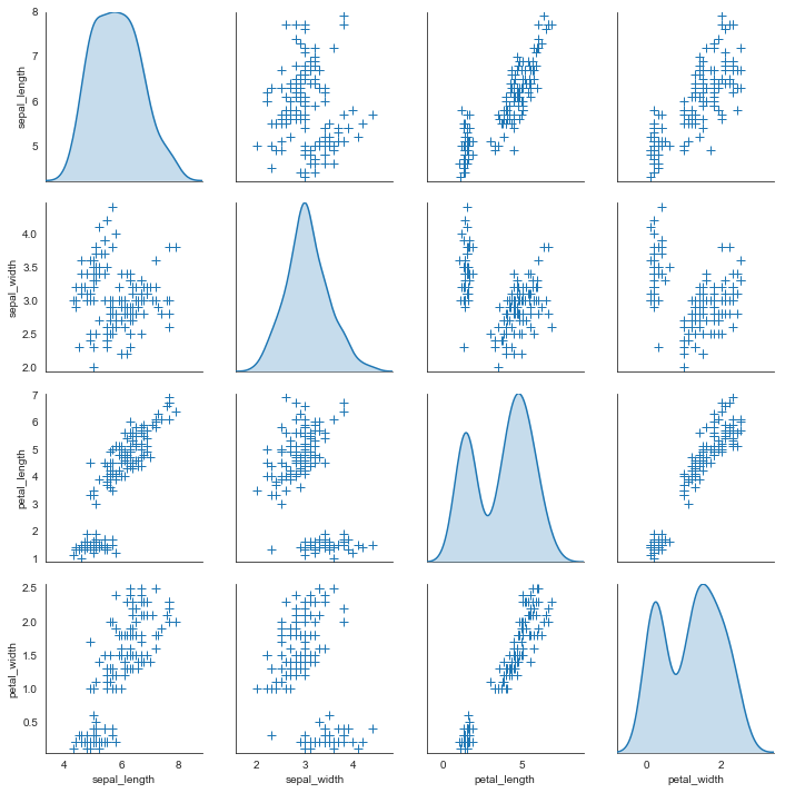
1 2 3 4 5 sns.pairplot(iris , diag_kind = 'kde' ,markers = '+' , plot_kws = dict (s = 50 ,edgecolor = 'b' ,linewidth = 1 ), diag_kws = dict (shade = True ))
<seaborn.axisgrid.PairGrid at 0x14feffb0>
1 2 3 4 5 6 7 8 9 10 11 12 13 14 15 16 17 18 19 20 g = sns.PairGrid(iris,hue = 'species' ,palette = 'hls' , vars = ['sepal_length' ,'sepal_width' ,'petal_length' ,'petal_width' ], size = 3 ) g.map_diag(plt.hist, histtype = 'barstacked' ,linewidth = 1 ,edgecolor = 'w' ) g.map_offdiag(plt.scatter,edgecolor = 'w' ,s = 40 ,linewidth = 1 ) g.add_legend()
<seaborn.axisgrid.PairGrid at 0x21652e90>
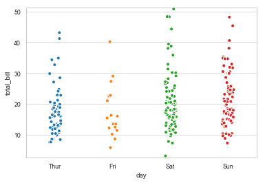
1 2 3 4 5 6 7 8 9 10 11 12 13 14 15 16 17 18 19 sns.set_style('whitegrid' ) sns.set_context('paper' ) tips = sns.load_dataset('tips' ) print (tips.head())sns.stripplot(x = 'day' , y = 'total_bill' , data = tips, jitter = True , size = 5 ,edgecolor = 'w' ,linewidth = 1 ,marker = 'o' )
   total_bill   tip     sex smoker  day    time  size
0       16.99  1.01  Female     No  Sun  Dinner     2
1       10.34  1.66    Male     No  Sun  Dinner     3
2       21.01  3.50    Male     No  Sun  Dinner     3
3       23.68  3.31    Male     No  Sun  Dinner     2
4       24.59  3.61  Female     No  Sun  Dinner     4

<matplotlib.axes._subplots.AxesSubplot at 0xc12130>
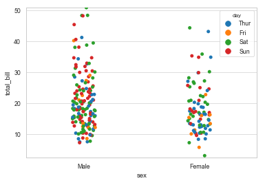
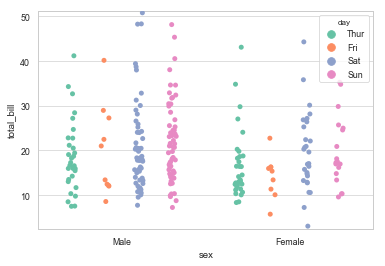
1 2 3 4 sns.stripplot(x = 'sex' ,y = 'total_bill' ,hue = 'day' , data = tips,jitter = True )
<matplotlib.axes._subplots.AxesSubplot at 0xf54fed0>
1 2 3 4 5 6 7 8 9 10 11 sns.stripplot(x = 'sex' ,y = 'total_bill' ,hue = 'day' , data = tips,jitter = True , palette = 'Set2' , dodge = True )
<matplotlib.axes._subplots.AxesSubplot at 0xf5524d0>
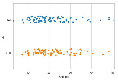
1 2 3 4 5 6 7 print (tips['day' ].value_counts())sns.stripplot(x = 'total_bill' ,y = 'day' ,data = tips,jitter = True , order = ['Sat' ,'Sun' ])
Sat     87
Sun     76
Thur    62
Fri     19
Name: day, dtype: int64

<matplotlib.axes._subplots.AxesSubplot at 0xb840b0>
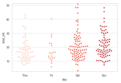
1 2 3 4 5 sns.swarmplot(x = 'day' ,y = 'total_bill' ,data = tips, size = 5 ,edgecolor = 'w' ,linewidth = 1 ,marker = 'o' , palette = 'Reds' )
<matplotlib.axes._subplots.AxesSubplot at 0xa53c70>
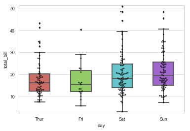
boxplot :又称为盒须图、盒式图或箱线图,是一种用作显示一组数据分散情况资料的统计图。因形状如箱子而得名
1 2 3 4 5 6 7 8 9 10 11 12 13 14 15 16 17 18 19 20 21 22 23 24 25 26 27 sns.set_style('whitegrid' ) sns.set_context('paper' ) tips = sns.load_dataset('tips' ) sns.boxplot(x = 'day' ,y = 'total_bill' ,data = tips, linewidth = 2 , width = 0.5 , fliersize = 3 , palette = 'hls' , whis = 1.5 , notch = False , order = ['Thur' ,'Fri' ,'Sat' ,'Sun' ])
1 <matplotlib.axes._subplots.AxesSubplot at 0x614e2b0>
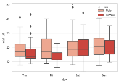
1 2 3 4 5 sns.boxplot(x = 'day' ,y = 'total_bill' ,data = tips,hue = 'sex' ,palette = 'Reds' )
1 <matplotlib.axes._subplots.AxesSubplot at 0x62316f0>
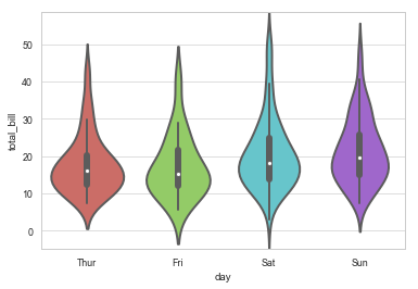
小提琴图其实是箱线图与核密度图的结合,通过小提琴图能更容易看出哪些位置的密度较高,即数据分布的区域
1 2 3 4 5 6 7 8 9 10 11 12 13 14 15 16 17 18 19 20 21 22 23 24 sns.violinplot(x = 'day' ,y = 'total_bill' ,data = tips, linewidth = 2 , width = 0.8 , palette = 'hls' , order = ['Thur' ,'Fri' ,'Sat' ,'Sun' ], scale = 'area' , gridsize = 50 , inner = 'box' , )
1 <matplotlib.axes._subplots.AxesSubplot at 0x10c7eab0>
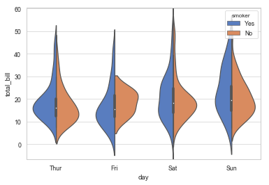
1 2 3 4 5 6 7 8 sns.violinplot(x = 'day' ,y = 'total_bill' ,data = tips, hue = 'smoker' ,palette = 'muted' , split = True , inner = 'box' )
1 <matplotlib.axes._subplots.AxesSubplot at 0x110572d0>
小提琴图结合散点图
1 2 3 4 5 sns.violinplot(x = 'day' ,y = 'total_bill' ,data = tips,palette = 'hls' ,inner = None ) sns.swarmplot(x = 'day' ,y = 'total_bill' ,data = tips,color = 'w' ,alpha = 0.5 )
1 <matplotlib.axes._subplots.AxesSubplot at 0x11224ed0>
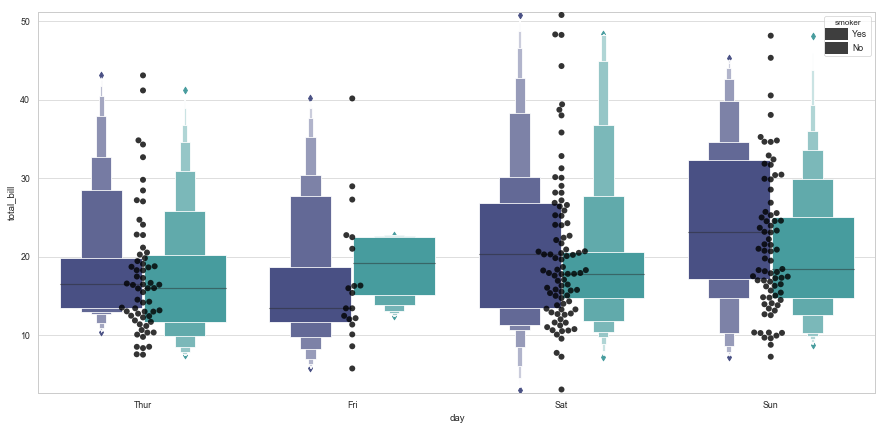
1 2 3 4 5 6 7 8 9 10 11 12 13 14 15 16 plt.figure(figsize = (15 ,7 )) sns.lvplot(x = 'day' ,y = 'total_bill' ,data = tips,palette = 'mako' , width = 0.8 , hue = 'smoker' , linewidth = 12 , scale = 'area' , k_depth = 'proportion' , ) sns.swarmplot(x = 'day' ,y = 'total_bill' ,data = tips,color = 'k' ,size = 6 ,alpha = 0.8 )
1 <matplotlib.axes._subplots.AxesSubplot at 0x11263f30>
这两篇博文列举了对数据分布情况的基础可视化图表,当然只是很基础的图表展示,记录下来以便随时翻阅,查漏补缺,还是那句话,任何图表可视化重点是数据结构与其逻辑,真正理解了数据才能更好的选择图表去展示,感谢阅读~
本文版权归作者所有,欢迎转载,转载请注明出处和链接来源。