摘要
根据销售额数据分析整个大型商场的销售情况,以及转化为可视化图表~
项目描述
项目名称:大型商场销售额分析及数据可视化
数据来源:该项目提供了从不同城市的10家商店中收集的1559种产品的2013年销售数据。
字段说明:
Item_Identifier : 唯一产品ID
Item_Weight : 产品重量
Item_Fat_Content : 产品是否低脂
Item_Visibility : 该产品占商店总产品展示区的百分比
Item_Type : 产品种类
Item_MRP : 产品最高零售价(标价)
Outlet_Identifier : 商品唯一ID
Outlet_Establishment_Year : 商品成立的年份
Outlet_Size : 商品的面积
Outlet_Location_Type : 商店所在城市类型
Outlet_Type : 商店的类型
项目目的:根据2013年的销售数据,通过可视化分析产品在不同维度的销售情况。
环境解释:基于jupyter notebook,可视化工具包:seaborn、matplotlib
1 | # 导入模块 |
1 | # 数据导入 |
数据分布
1 | # 查看Item_Outlet_Sales项的数据分布情况 |
<matplotlib.axes._subplots.AxesSubplot at 0x1a2431c860>
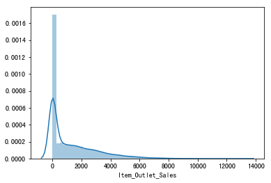
1 | # 查看偏度系数、峰度系数 |
偏度系数Skewness: 1.544684
峰度系数Kurtsis: 2.419439
图表解析:
输出结果可以看出:1、偏离正态分布;2、具有明显的正偏态
注意:原先将测试数据里的Item_Outlet_Sales项全赋值为0
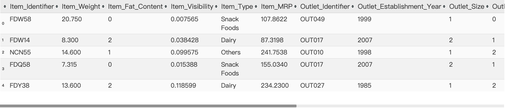
数据查看
1 | # 查看训练数据的数值变量的描述统计 |
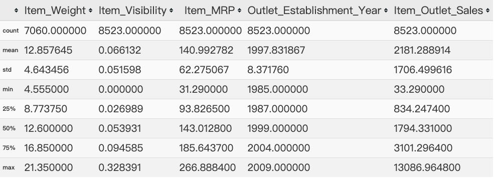
图表解析:
1、Item_Visibility的最小值为零。这没有实际意义,因为当在商店中销售产品时,可见性不能为0。
2、Outlet_Establishment_Years从1985年到2009年各不相同。这种形式的值可能不合适。
相反,如果我们可以将它们转换为特定商店的年龄,它应该对销售产生更好的影响。
1 | # 检查各列缺失值 |
Item_Identifier                 0
Item_Weight                  2439
Item_Fat_Content                0
Item_Visibility                 0
Item_Type                       0
Item_MRP                        0
Outlet_Identifier               0
Outlet_Establishment_Year       0
Outlet_Size                  4016
Outlet_Location_Type            0
Outlet_Type                     0
source                          0
Item_Outlet_Sales               0
dtype: int64
图表解析:Item_Weight和Outlet_Size存在缺失值
1 | # 查看每个变量的唯一值 |
Item_Identifier               1559
Item_Weight                    416
Item_Fat_Content                 5
Item_Visibility              13006
Item_Type                       16
Item_MRP                      8052
Outlet_Identifier               10
Outlet_Establishment_Year        9
Outlet_Size                      4
Outlet_Location_Type             3
Outlet_Type                      4
source                           2
Item_Outlet_Sales             3494
dtype: int64
图表解析:一共有1559种产品和十个商店,值得注意的是:Item_Type有16个唯一值
1 | # 查看每个字段中不同类别的频率统计 |
Frequency of Categories for varible Item_Fat_Content
Low Fat    8485
Regular    4824
LF          522
reg         195
low fat     178
Name: Item_Fat_Content, dtype: int64

Frequency of Categories for varible Item_Type
Fruits and Vegetables    2013
Snack Foods              1989
Household                1548
Frozen Foods             1426
Dairy                    1136
Baking Goods             1086
Canned                   1084
Health and Hygiene        858
Meat                      736
Soft Drinks               726
Breads                    416
Hard Drinks               362
Others                    280
Starchy Foods             269
Breakfast                 186
Seafood                    89
Name: Item_Type, dtype: int64

Frequency of Categories for varible Outlet_Identifier
OUT027    1559
OUT013    1553
OUT046    1550
OUT049    1550
OUT035    1550
OUT045    1548
OUT018    1546
OUT017    1543
OUT010     925
OUT019     880
Name: Outlet_Identifier, dtype: int64

Frequency of Categories for varible Outlet_Size
Medium    4655
Small     3980
High      1553
Name: Outlet_Size, dtype: int64

Frequency of Categories for varible Outlet_Location_Type
Tier 3    5583
Tier 2    4641
Tier 1    3980
Name: Outlet_Location_Type, dtype: int64

Frequency of Categories for varible Outlet_Type
Supermarket Type1    9294
Grocery Store        1805
Supermarket Type3    1559
Supermarket Type2    1546
Name: Outlet_Type, dtype: int64
图表解析:
1、Item_Fat_Content:有Low Fat、LF和low fat,以及Regular和reg的数据
2、Outlet_Type:type2和type3的数据过少,是否需要合并为一个类别
数据清洗
数据待处理:
- Item_Visibility的最小值为零。这没有实际意义,因为当在商店中销售产品时,可见性不能为0。
- Outlet_Establishment_Years从1985年到2009年各不相同。这种形式的值可能不合适。相反,如果我们可以将它们转换为特定商店的年龄,有可能对销售预测产生更好的影响。
- Item_Weight和Outlet_Size存在缺失值
- Item_Fat_Content:有Low Fat、LF和low fat,以及Regular和reg的数据
- Outlet_Type:type2和type3的数据过少,是否需要合并为一个类别
数据重定义
1 | # 我们注意到 Item_Visibility 的最小值是0,这没有实际意义。让我们把它看作是丢失的信息,并将其与产品的平均可见性联系起来。 |
number of 0 values initially: 879
number of 0 values after modification: 0
缺失值填充
1 | # Item_Weight缺失值:可以考虑用重量平均数填充 |
Orignal #missing: 2439
Final #missing: 0
1 | # outlet_size缺失值处理:关于商店的面积因为没有相对的参数去评估,所以这里使用scipy中的mode模块来处理,即用众数来替换空值 |
Mode for each Outlet_Type:
Outlet_Type Grocery Store Supermarket Type1 Supermarket Type2  \
Outlet_Size           nan             Small            Medium

Outlet_Type Supermarket Type3
Outlet_Size            Medium

Orignal #missing: 4016
Final #missing: 0
问题发现:可以发现Outlet_Size中有nan值存在,数据量有925条,观察数据,可选择将nan值暂定处理为Medium
1 | data['Outlet_Size'].replace('nan','Medium',inplace = True) |
Small     7071
Medium    5580
High      1553
Name: Outlet_Size, dtype: int64
数据整合
1 | # 处理Item_Fat_Content(产品是否低脂)数据存在别名的情况 |
Low Fat    9185
Regular    5019
Name: Item_Fat_Content, dtype: int64
1 | # 新特征生成 |
Food              10201
Non-Consumable     2686
Drink              1317
Name: Item_Type_Combined, dtype: int64
1 | # 因为上一步根据唯一ID将产品分为三大类,而类别中有Non-Consumable(非消耗品),可以考虑根据这个类别将是否低脂选项进行细分 |
Low Fat       6499
Regular       5019
Non-Edible    2686
Name: Item_Fat_Content, dtype: int64
可视化
商店面积
1 | # 商店面积类别柱状图 |
<matplotlib.axes._subplots.AxesSubplot at 0x1a25636cf8>
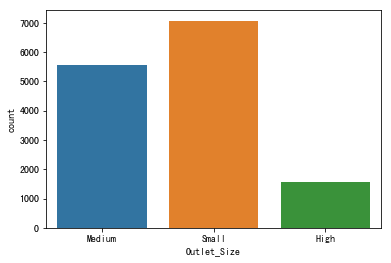
图表解析:可看出大部分都属于中小型商店,大型商店占比较小
商品是否低脂与产品重量
1 | # 商品是否低脂与产品重量 |
<matplotlib.axes._subplots.AxesSubplot at 0x1a25b12da0>
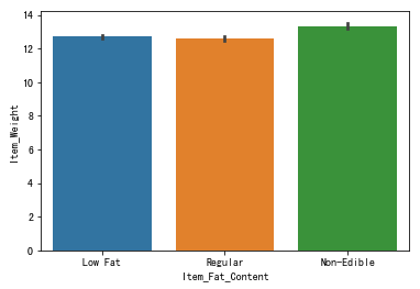
图表解析:可以看出商品是否低脂与产品重量没什么多大联系
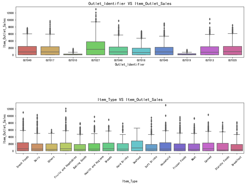
商店ID与销售额
1 | # Outlet_Identifier 与 Item_Outlet_Sales |
<matplotlib.axes._subplots.AxesSubplot at 0x1a25ae9550>
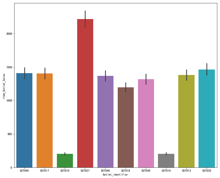
图表解析:OUT017与OUT019的销售额最少,经营情况很差;而OUT027的销售额最高,其余商店的销售额相差无几
商品种类与销售额
1 | # 商品种类与销售额趋势图 |
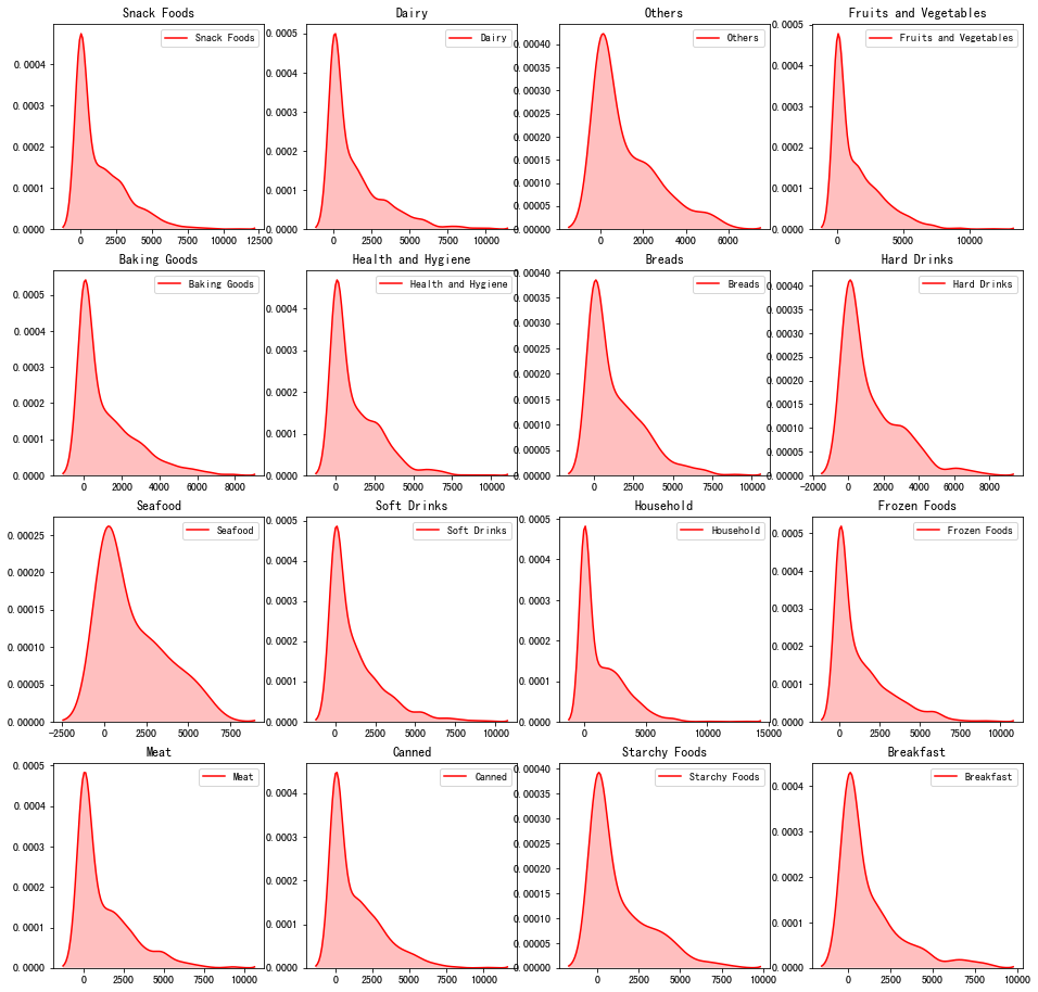
图表解析:明显可以看出,Seafood的销售金额相比其他会高出不少,而Fruits and Vegetables的销售金额曲线最平滑,金额也偏低。
商店ID与销售额
1 | # Outlet_Identifier 与 销售额 |
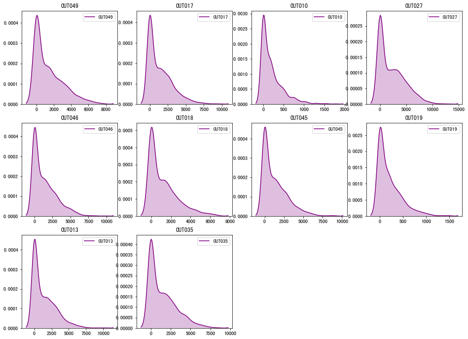
图表解析:与上面分析结果一致,销售额最差的是OUT017与OUT019,经营情况最差;而销售额最高的是OUT027,其余商店销售额曲线相差不大
商店年份与销售额
1 | data.groupby('Outlet_Establishment_Year')['Item_Outlet_Sales'].mean().plot.bar() |
(array([0, 1, 2, 3, 4, 5, 6, 7, 8]), <a list of 9 Text xticklabel objects>)
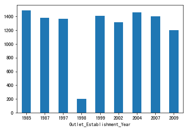
图表解析:可以看出除1998年,其他商店年份的销售额都相差不大
商店年龄与销售额
1 | # 定义新特征 - 将年份转变成商店年龄 |
(array([0, 1, 2, 3, 4, 5, 6, 7, 8]), <a list of 9 Text xticklabel objects>)
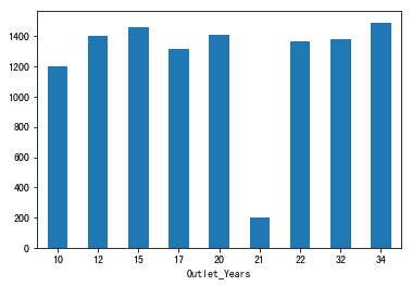
1 | plt.figure(figsize = (12,6)) |
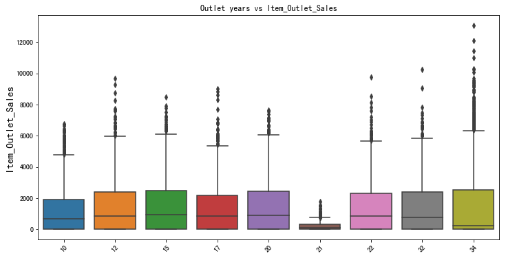
图表解析:商店年龄在21年的商店销售额最少
商品类别、商品是否低脂与销售额
1 | # 原先考虑将超市Type2和Type3变量 |
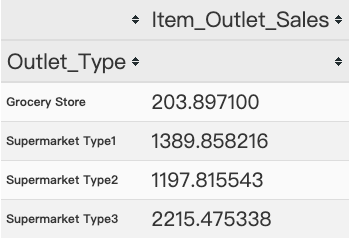
图表解析:可以看出销售额存在差异,所以我们保留两个特征
1 | # Item_Type_Combined 、Item_Fat_Content 箱型图 |
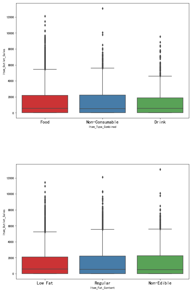
图表解析:Drink类商品的销售额相比另外两种还是要差上不少,而商品是否低脂与销售额基本上关系不大,与上面的分析结果一致
商店ID与产品种类
1 | # Outlet_Identifier 、Item_Type 箱型图 |
数据类型转换
1 | # 因为由于scikit-learn只接受数值变量,所以我将所有类别的名义变量类别转换为数值类型。 -- 进行标准化 |
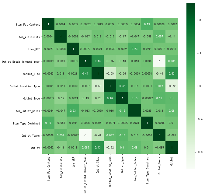
相关性 - 热力图
1 | # 标准化后查看训练数据的各项相关性 |
独热编码
1 | #One Hot Coding: |
1 | data.dtypes |
Item_Identifier               object
Item_Weight                  float64
Item_Visibility              float64
Item_Type                     object
Item_MRP                     float64
Outlet_Identifier             object
Outlet_Establishment_Year      int64
source                        object
Item_Outlet_Sales            float64
Outlet_Years                   int64
Item_Fat_Content_0             uint8
Item_Fat_Content_1             uint8
Item_Fat_Content_2             uint8
Outlet_Location_Type_0         uint8
Outlet_Location_Type_1         uint8
Outlet_Location_Type_2         uint8
Outlet_Size_0                  uint8
Outlet_Size_1                  uint8
Outlet_Size_2                  uint8
Outlet_Type_0                  uint8
Outlet_Type_1                  uint8
Outlet_Type_2                  uint8
Outlet_Type_3                  uint8
Item_Type_Combined_0           uint8
Item_Type_Combined_1           uint8
Item_Type_Combined_2           uint8
Outlet_0                       uint8
Outlet_1                       uint8
Outlet_2                       uint8
Outlet_3                       uint8
Outlet_4                       uint8
Outlet_5                       uint8
Outlet_6                       uint8
Outlet_7                       uint8
Outlet_8                       uint8
Outlet_9                       uint8
dtype: object
数据保存
1 | # 删除一些不必要项 |
未完待续
总结
以上是大型商店销售额预测项目的一些分析以及可视化,原项目是为做预测模型来预测各个商店的未来的经营情况,本次只做了一下商店数据上的分析以及可视化,算法部分有心无力,待学成再补充,有任何需要修正的地方,欢迎指正,感谢阅读~